SMA* ( Simplified Memory Bounded A*) is a shortest path algorithm that is based on the A* algorithm. The difference between SMA* and A* is that SMA* uses a bounded memory, while the A* algorithm might need exponential memory.
Like the A*, it expands the most promising branches according to the heuristic. What sets SMA* apart is that it prunes nodes whose expansion has revealed less promising than expected.
SMA*, just like A* evaluates nodes by combining g(n), the cost to reach the node, and h(n), the cost to get from the node to the goal: f(n) = g(n) + h(n).
Since g(n) gives the path cost from the start node to node n, and h(n) is the estimated cost of the cheapest path from n to the goal, we have f(n) = estimated cost of the cheapest solution through n. The lower the f value is, the higher priority the node will have.
The difference from A* is that the f value of the parent node will be updated to reflect changes to this estimate when its children are expanded. A fully expanded node will have an f value at least as high as that of its successors.
In addition, the node stores the f value of the best forgotten successor (or best forgotten child). This value is restored if the forgotten successor is revealed to be the most promising successor.
Before continuing reading this post, we suggest you read our post on the A* algorithm. Understanding how A* works will help you a lot in understanding how SMA* works.
Visual representation of how Simplified Memory Bounded A* (SMA*) works:
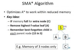
Image 1: Idea of how SMA* works
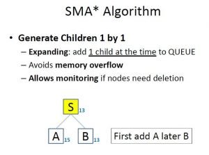
Image 2: Generating Children in SMA* Algorithm

Image 3: Handling Long Paths i.e. Too Many Nodes In The Memory
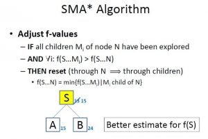
Image 4: Adjusting The f Value
Problem
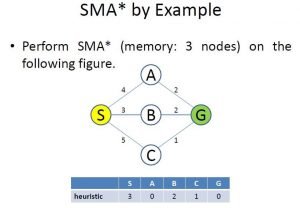
Image 5: The Problem of Simplified Memory Bounded A*
On Image 5 we have the problem we are about to solve. Our requirement is to find the shortest path starting from node “S” to node “G”. We can see the graph and how the nodes are connected. Also, we can see the table, containing the heuristic values for each of the nodes.
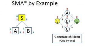
Image 6: Evaluating The Children
On Image 6 we can see how the algorithm evaluates the children. Firstly it added the “A” and “B” nodes (starting alphabetically). On the right of the node in blue color is the f value, on the left is the g value or the cost to reach that node(in green color), and the h value or the heuristic (in red color).
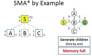
Image 7: Full Memory While Evaluation
On Image 7 we can see what happens when you want to evaluate more nodes than what the memory allows. The already evaluated children with the highest f value get removed, but its value is remembered in its parent(the number in purple color on the right of the “S” node).

Image 8: Adjusting The f Value
On Image 8 we can see that if all accessible children nodes are visited or explored we adjust the parent’s f value to the value of the children with the lowest f value.

Image 9: Memory Full Evaluate Through The Lowest f Value Child
On Image 9 we can see how the algorithm evaluates the children of the “A” node. The only children is the “G” node which is the goal, which means there is now a way for exploring further.
Now we remove the “C” node, since it has the highest f value but we don’t remember it, since the “B” node has a lower value. Now we update the f value of the “A” node to 6 because all the children accessible are explored.

Image 10: Update The Root Value (“S” node) To The Remembered Value
Just because we’ve reached the goal node, doesn’t mean that the algorithms are finished. As we can see the remembered f value of the “B” node is lower than the f value of the “G” node explored through the “A” node.
This gives hope that we might reach the goal node again for a lower f value or lower total cost. We also update the f value of the “S” node to 5 since there is no more child node with value 4.

Image 11: Remove The Goal Leading Node
As we can see on Image 11 we will remove the “A” node since it has already discovered the goal and has the same f value as the “C” node so we will remember this node in the parent “S” node.
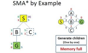
Image 12: Reaching The Goal For The Lowest Total Cost
On Image 12 we can see that we’ve reached the goal again, this time through the “B” node. This time cost is lower than through the “A” node.
The memory is full, which means we need to remove the “C” node, because it has the highest f value, and it means that if we eventually reach the goal from this node the total cost at best case scenario will be equal to 6, which is worse than we already have.
At this stage, the algorithm terminates, and we have found the shortest path from the “S” node to the “G” node.
Conclusion
SMA* (Simplified Memory Bounded A Star) is a very popular graph pathfinding algorithm, mainly because it is based on the A* algorithm, which already does a very good job of exploring the shortest path in graphs. This algorithm is better than A* because it is memory-optimized.
As in the A* post, we cannot end this post without saying how important is the understanding of this algorithm if you want to continue to learn about more complex graph searching algorithms.
Like with every post we do, we encourage you to continue learning, trying and creating.