Gradient descent is an iterative optimization algorithm for finding a local minimum of a differentiable function. To find a local minimum of a function using gradient descent, we take steps proportional to the negative of the gradient (or approximate gradient) of the function at the current point. But if we instead take steps proportional to the positive of the gradient, we approach a local maximum of that function.
Gradient descent is also known as steepest descent, but gradient descent should not be confused with the method of steepest descent for approximating integrals.
Suppose you are lost in the mountains in a dense fog, you can only feel the slope of the ground below your feet. A good strategy to get to the bottom of the valley quickly is to go downhill in the direction of the steepest slope.
This is exactly what Gradient Descent does, it measures the local gradient of the error function with regards to the parameter vector θ, and it goes in the direction of descending gradient. Once the gradient is zero, you have reached a minimum!
An important parameter in Gradient Descent is the size of the steps, determined by the learning rate hyperparameter.
If the learning rate is too small, then the algorithm will have to go through many iterations to converge, which will take a long time.
If the learning rate is too high, it might make the algorithm diverge, with larger and larger values, failing to find a good solution.
Types of Gradient Descent in Python
Batch Gradient Descent
Batch gradient descent (BGD) computes the gradient using the whole dataset. This is great for convex, or relatively smooth error manifolds. In this case, we move somewhat directly towards an optimum solution.
To implement Gradient Descent, you need to compute the gradient of the cost function with regards to each model parameter θj. In other words, you need to calculate how much the cost function will change if you change θj just a little bit. This is called a partial derivative.
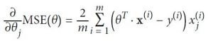
Image 1: Partial derivatives of the cost function
On Image 1, we can see the equation that calculates the partial derivatives of the cost function (MSE cost function in this example) for parameter θj.
Since we are going to use the whole dataset, we can create a vector of all of that data so we don’t need to calculate the gradients individually. The vector will contain all of the partial derivatives of the function.
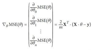
Image 2: The gradient vector of the cost function
On Image 2 we have the equation for the Gradient vector of the MSE cost function.
Now let’s get back to the example where we are trying to get to the bottom of the valley. We have the vector which points up the valley, we need to go opposite of the vector. With the following equation, we are calculating the step we need to take.
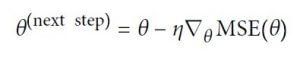
Image 3: Gradient descent next step
On Image 3 we have the formula that calculates the next step. We subtract the product of the learning rate η and the partial derivate on step θ from the current step θ.
import numpy as np
X = 2 * np.random.rand(100, 1)
y = 4 + 3 * X + np.random.randn(100, 1)
X_b = np.c_[np.ones((100, 1)), X]
eta = 0.1 # learning rate
n_iterations = 1000
m = 100
theta_best = np.linalg.inv(X_b.T.dot(X_b)).dot(X_b.T).dot(y)
print(“THE BEST THETA VALUE IS: “, theta_best)
theta = np.random.randn(2,1) # random initialization
for iteration in range(n_iterations):
gradients = 2/m * X_b.T.dot(X_b.dot(theta) – y)
theta = theta – eta * gradients
print(“Theta for iteration”,iteration,” is: “,theta)
print(“Theta result:”, theta)
This is the code that will determine the value for the θ parameter. As you can see we are using linear regression as well so we can compare the results.
The linear regression result is theta_best variable, and the Gradient Descent result is in theta variable. We are using the data y = 4 + 3*x + noise.
If you don’t know how Linear Regression works and how to implement it in Python please read our article about Linear Regression with Python.
What we need to compare is the theta_best and theta variables values to see if our gradient descent has good value determination for θ parameter.
The Linear Regression result is:
THE BEST THETA VALUE IS: [[3.63788102][3.15461233]]
The Gradient Descent result is:
Theta result: [[3.63788102][3.15461233]]
As we can see the values are the same, which means our Gradient Descent model works fine. This is a result of a good learning rate. But what happens if we change the learning rate?
η=0.01
Linear Regression:
THE BEST THETA VALUE IS: [[4.15971718][2.84269615]]
Gradient Descent:
Theta result: [[4.07012587][2.91529257]]
η=0.50
Linear Regression:
THE BEST THETA VALUE IS: [[4.16071641][2.78866131]]
Gradient Descent:
Theta result: [[-1.10637101e+13][-1.20809572e+13]]
η=0.25
Linear Regression:
THE BEST THETA VALUE IS: [[3.9554697 ][2.99551949]]
Gradient Descent:
Theta result: [[3.9554697 ][2.99551949]]
From the three different values, only for a learning rate of 0.25, we have the same theta values from the Linear Regression and the GradientDescent models. But we cannot always experiment with the learning rate, there must be a way that we can determine it. And yes there is, it is called grid search. Here you can find how to use it.
Stochastic Gradient Descent
Stochastic gradient descent (SGD) computes the gradient using a single sample. Most applications of SGD actually use a minibatch of several samples. SGD works better than batch gradient descent for error manifolds that have lots of local maxima/minima.
In this case, the somewhat noisier gradient calculated using the reduced number of samples tends to jerk the model out of local minima into a region that hopefully is more optimal.
Single samples are really noisy, while minibatches tend to average a little of the noise out. Thus, the amount of jerk is reduced when using minibatches.
A good balance is struck when the minibatch size is small enough to avoid some of the poor local minima, but large enough that it doesn’t avoid the global minima or better-performing local minima.
Randomness of SGD is good to escape from local optima, but bad because it means that the algorithm can never settle at the minimum. One solution to this dilemma is to gradually reduce the learning rate.
The steps start out large (which helps make quick progress and escape local minima), then get smaller and smaller, allowing the algorithm to settle at the global minimum.
The function that determines the learning rate at each iteration is called the learning schedule. If the learning rate is reduced too quickly, you may get stuck in a local minimum.
If the learning rate is reduced too slowly, you may jump around the minimum for a long time and end up with a suboptimal solution if you halt training too early.
n_epochs = 50
t0, t1 = 5, 50 # learning schedule hyperparameters
def learning_schedule(t):
return t0 / (t + t1)
theta_sgd = np.random.randn(2,1) # random initialization
for epoch in range(n_epochs):
for i in range(m):
random_index = np.random.randint(m)
xi = X_b[random_index:random_index+1]
yi = y[random_index:random_index+1]
gradients = 2 * xi.T.dot(xi.dot(theta_sgd) – yi)
eta = learning_schedule(epoch * m + i)
theta_sgd = theta_sgd – eta * gradients
print(“Theta for iteration”, i, ” is: “, theta_sgd)
print(“Theta SGD result is: “,theta_sgd)
Linear Regression:
THE BEST THETA VALUE IS: [[4.13015408][3.05577441]]
Batch Gradient Descent:
Theta result: [[4.13015408][3.05577441]]
Stochastic Gradient Descent:
Theta SGD result is: [[4.16106047][3.07196655]]
Above we have the code for the Stochastic Gradient Descent and the results of the Linear Regression, Batch Gradient Descent and the Stochastic Gradient Descent.
As we can see SGD iterated through the whole training set only 50 times (in each epoch) while the BGD iterated 1000 times. As we can see it has quite good results when we compare the numbers of iterations.
If you don’t want to write all of those lines of code you can use scikit-learn model that will help you to do SGD in a few lines of code.
from sklearn.linear_model import SGDRegressor
sgd_reg = SGDRegressor(n_iter=50, penalty=None, eta0=0.1)
sgd_reg.fit(X, y.ravel())
print(“Theta SGD scikit-learn result is: “, [sgd_reg.intercept_[0], sgd_reg.coef_[0]])
Linear Regression:
THE BEST THETA VALUE IS: [[4.13498897][2.97196157]]
Batch Gradient Descent:
Theta result: [[4.13498897][2.97196157]]
Stochastic Gradient Descent:
Theta SGD result is: [[4.007083 ][2.94810673]]
Stochastic Gradient Descent Scikit-Learn:
Theta SGD scikit-learn result is: [4.127058183692392, 2.970673440517907]
As we can see from the results again the SGD results are very close to the Linear Regression and BGD results.
Conclusion
Gradient Descent is one of the most popular optimization strategies and it is widely used in many Machine Learning and Deep Learning models.
It is very important for every Machine Learning Engineer and Data Scientist to know how to implement this strategy and how to use it properly.
There are more complex and better optimization techniques that Gradient Descent, but in order to understand those, you need to understand Gradient Descent first.
Our suggestion is to find a problem where you need to determine the value of a parameter and try to translate it to code (Python, C++ or R) and use Gradient Descent to find that parameter’s value.
This way you will understand it the best since you’ve tried it on a real-world problem.
Like with every post we do, we encourage you to continue learning, trying and creating.