
If you want to get familiar with Artificial Neural Networks, which are the base of Deep Learning, one of the most popular and promising branches of Machine Learning.
In this post, we will try to give you the most information about Artificial Neural Networks in the shortest possible time range. That’s because our goal is to educate interested individuals, without taking too much of their freedom.
In this post you will get familiar with:
- Working details of neural networks
- The impact of various hyperparameters on neural networks
- Feed-forward and backpropagation
- Practical implementation of Artificial Neural Networks with Python
If you are a frequent visitor to our website, you’ve probably already read our other articles about FREE courses from some of the top universities or companies. If you haven’t here are some of them:
- FREE Computer Science Curriculum From The Best Universities and Companies In The World
- Top 40 COMPLETELY FREE Coursera Artificial Intelligence and Computer Science Courses
- How To Become a Certified Data Scientist at Harvard University for FREE
- How to Gain a Computer Science Education from MIT University for FREE
- Top 50 FREE Artificial Intelligence, Computer Science, Engineering and Programming Courses from the Ivy League Universities
- Top 10 Best FREE Artificial Intelligence Courses from Harvard, MIT, and Stanford
What are Artificial Neural Networks
Artificial Neural Networks (ANN) are computing systems that are inspired by, biological neural networks that constitute animal brains. Such systems “learn” to perform tasks by considering examples, generally without being programmed with task-specific rules.
They belong to the family of supervised learning algorithms. The Artificial Neural Network leverages a mix of multiple hyperparameters that help in approximating complex relations between input and output.
In order to get better precision in determining the output from the given input, usually, we combine the hyperparameters in the different stages of the process of working with an ANN.
The most popular and most used hyperparameters are used in working with the ANNs are: number of hidden layers, number of hidden units, activation function, learning rate.
Structure of an Artificial Neural Network

Image 1: Visual representation of a structure of an Artificial Neural Network
On Image 1, is represented the structure of the Artificial Neural Network, so you can get a visual representation of what they look like.
As we can see the first elements of the structure belong to the Input layer. These elements represent the input in the neural network, or the dependent variables (if you are familiar with regression). Based on the values of these input variables we want to predict the output of this network.
After the input layer, we have two hidden layers (the number of these layers is not static, but we must determine the right number of hidden layers in order to avoid complexity which can result in overfitting).
In this layer, we are using different activation functions on the input values so we can create a better classification for the out results.
The last layer is the output layer. As we can see here, in our output we have two values. The number of values is dependent on the number of classes we have.
How to train an Artificial Neural Network
Training a neural network basically means calibrating all the weights by repeating two steps, forward propagation, and backpropagation.
Forward propagation is applying a set of weights to the input data and calculate an output.
For the first forward propagation, the set of weights values are initialized randomly.
Backpropagation is measuring the margin of error of the output and adjusts the weights accordingly to decrease the error.
We will repeat both of these steps until the weights are calibrated to accurately predict an output.
How Forward Propagation works
To understand how forward propagation works, we can use the next example.
| Input | Output |
|---|---|
| (0,0) | 0 |
| (0,1) | 1 |
| (1,0) | 1 |
| (1,1) | 0 |
In the table, we have two columns representing the input variables (two values), and the output represented with one variable (one value).
If you did not figure out until now, the function we use to get the output is nothing more than the logical operation XOR. Forward propagation will call this function on every layer after the input layer, until it produces some values for the output.
For example, if we have a neural network with 2 hidden layers, the values of the input layer and the function will produce output values for the first hidden layer. Then these values and the function will produce output values for the second hidden layer, and then the values of the second hidden layer (which was the output of the values of the first hidden layer and the function) and the function will produce the final output values in the output layer.

Image 2: Visual representation of how Forward Propagation works
On Image 2, we have a representation of how Forward Propagation works. As we can see, we have the input, which consists of two dependent variables, and both of them consist of the value equal to 1.
Every of the input nodes is connected to every node in the hidden layer. Each of the connections is joined by a weight value, that will help the network to determine the output with higher precision. As we said before, in the first epoch of training, these weights are randomly selected.
All of the nodes in the hidden layer are connected to the node in the output layer. Those connections are also joined by weight values.
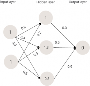
Image 3: Values for the hidden layer
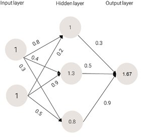
Image 4: The output value of the network.
On Image 3 and Image 4 are represented the values after the first epoch of training that the nodes in the hidden and output layers get respectively.
These values are calculated following the formula in Image 5.
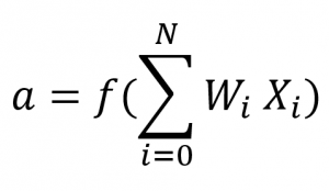
Image 5: Activation function
The formula in Image 5 is called an activation function and is used to calculate the value of each node. By calculating the sum of the products of every node from the previous layer and the weight by which that node is connected to the node we want to calculate the value for.
1 x 0.8 + 1 x 0.2 = 1
1 x 0.4 + 1 x 0.9 = 1.3
1 x 0.3 + 1 x 0.5 = 0.8
Activation functions
As we mentioned in the previous section, in the hidden layers we are using activation functions, that will predict the output with the highest possible precision.
There are different activation functions. Well, one of the most popular activation functions are: Sigmoid, Relu, Tanh, etc.
In this post we are going to use the Sigmoid activation function to the previous example, to show you the difference in the values for one training epoch.
The Sigmoid function takes the form 1 / ( 1 + e-x ) where “x” stands for the value of the node, calculated the same way as we did the calculation in the previous section.

Image 6: Hidden layer and output layer nodes values using Sigmoid function.
1 x 0.8 + 1 x 0.2 = 1
1 x 0.4 + 1 x 0.9 = 1.3
1 x 0.3 + 1 x 0.5 = 0.8
Sigmoid(1.0) = 0.731
Sigmoid(1.3) = 0.785
Sigmoid(0.8) = 0.689
0.73 x0.3 + 0.79 x0.5 + 0.69 x 0.9 = 1.235
After each session, we need to calculate the error, which is the difference between the predicted value, and the value we actually want to get as an output.
The error can be calculated in a different way. We are going to use the squared error, which is the calculated difference but squared.
How backpropagation works
In forward propagation, we took a step from input to hidden to output. In backpropagation, we take the reverse approach: essentially, change each weight starting from the last layer by a small amount until the minimum possible error is reached.
When weight is changed, the overall error either decreases or increases. Depending on whether the error increased or decreased, the direction in which a weight is updated is decided.
Moreover, in some scenarios, for a small change in weight, error increases/decreases by quite a bit, and in some cases, error changes only by a small amount.
A big role when we are doing backpropagation plays the learning rate. The learning rate helps us in building trust in our decision of weight updates.
For example, while deciding on the magnitude of weight update, we would potentially not change everything in one go but rather take a more careful approach in updating the weights more slowly. This results in obtaining stability in our model.
The way that the weight is updated is by following the next formulas:
δtarget = y(1-y)(ytarget-y) – this is the formula for calculating the δ value of the target node. δ is used in updating the weight. y is the predicted value.
δhidden_layer = yi(1-yi)wijδj – this is the formula for calculating the δ value of a node in the hidden layer.
δ is used in updating the weight on the nodes in the hidden layer that comes before this layer (looking from the input layer).
yi is the predicted value, for the current node, wij is the weight of the connection between this node and the node in the layer after the current layer.
δj is the δ value for the node of the next layer, connected with the current node with the weight wij.
wij = ηδj yi – this is the formula for updating the weight between a node that belongs to the i-th layer and a node that belongs to the j-th layer.
yi is the predicted value, for the current node, δj is the value of a j-th node, and η is the learning rate.
Practical implementation of neural network with Python
For this example we are going to use the keras-mnist dataset. MNIST contains 70000 images of handwritten digits: 60000 for training and 10000 for testing. The images are grayscale, 28×28 pixels, and centered to reduce preprocessing and get started quicker.
from keras.datasets import mnist
import matplotlib.pyplot as plt
from keras.models import Sequential
from keras.layers import Dense
from keras.utils import np_utils
(X_train, y_train), (X_test, y_test) = mnist.load_data()
# plot 4 images as gray scale
plt.subplot(221)
plt.imshow(X_train[0], cmap=plt.get_cmap(‘gray’))
plt.subplot(222)
plt.imshow(X_train[1], cmap=plt.get_cmap(‘gray’))
plt.subplot(223)
plt.imshow(X_train[2], cmap=plt.get_cmap(‘gray’))
plt.subplot(224)
plt.imshow(X_train[3], cmap=plt.get_cmap(‘gray’))
# show the plot
plt.show()
num_pixels = X_train.shape[1] * X_train.shape[2]
# reshape the inputs so that they can be passed to the vanilla NN
X_train = X_train.reshape(X_train.shape[0],num_pixels).astype(‘float32’)
X_test = X_test.reshape(X_test.shape[0],num_pixels).astype(‘float32’)
# scale inputs
X_train = X_train / 255
X_test = X_test / 255
# one hot encode the output
y_train = np_utils.to_categorical(y_train)
y_test = np_utils.to_categorical(y_test)
num_classes = y_test.shape[1]
# building the model
model = Sequential()
# add 1000 units in the hidden layer. Apply relu activation in hidden layer
model.add(Dense(1000, input_dim=num_pixels,activation=‘relu’))
# initialize the output layer
model.add(Dense(num_classes, activation=‘softmax’))
# compile the model
model.compile(loss=‘categorical_crossentropy’,
optimizer=‘adam’, metrics=[‘accuracy’])
# extract the summary of model
model.summary()
#run the model
model.fit(X_train, y_train, validation_data=(X_test, y_test), epochs=5, batch_size=1024, verbose=1)

Image 7: The accuracy of the model in each of the 5 epochs of training.
From this example, we can see that it took us not a lot of time to have a precision of 97.31% in classifying handwritten digit.
Conclusion
As we can see, this post is just a glimpse of what neural networks are and how forward propagation and backpropagation works. We hope that we sparked a little interest in you, so you can continue to learn more stuff and techniques that will help you manipulate these structures, and use their real power.