The iPhone is Apple’s most famous product bringing huge revenue to the company and its investors. The iPhone brings a huge community to Apple, creating perfect conditions for the company to increase the sales of the other products, like iMac, iMac Pro, MacBook Air, MacBook Pro, Mac Mini, etc.
All of these devices share one thing, the operating system, more precisely the nature of their operating systems. The iPhones and the iPads and the iWatches are running on iOS and their laptops and desktop computers are running on МacOS.
The common things for these operating systems are that the native apps for both of them need to be written in Objective-C or Swift.
In this article, we are going to talk about Swift, or more precisely, how to do Machine Learning with Swift, that will help you produce cutting edge modern apps for the iPhone, MacBook, etc. Here’s how to become Machine Learning Specialist in under 20 hours with a free course.
Wikipedia: “Swift is a general-purpose, multi-paradigm, compiled programming language developed by Apple Inc. and the open-source community, first released in 2014. Swift was developed as a replacement for Apple’s earlier programming language Objective-C, as Objective-C had been largely unchanged since the early 1980s and lacked modern language features.
Swift works with Apple’s Cocoa and Cocoa Touch frameworks, and a key aspect of Swift’s design was the ability to interoperate with the huge body of existing Objective-C code developed for Apple products over the previous decades.
It is built with the open-source LLVM compiler framework and has been included in Xcode since version 6, released in 2014. On Apple platforms, it uses the Objective-C runtime library which allows C, Objective-C, C++, and Swift code to run within one program.”
Don’t forget to read our latest and similar articles:
- You Can Now Learn for FREE: 9 Courses by Google about Artificial Intelligence, Machine Learning and Data Science
- Top 40 COMPLETELY FREE Coursera Artificial Intelligence and Computer Science Courses
- Unbelievable: You Can Now Build a Natural Language Processing Question Answering System in LESS Than 20 Lines of Code
- This is the Future of Artificial Intelligence: Deep Learning with JavaScript, Node.js, and TensorFlow
Create your first Machine Learning project with Swift and TensorFlow for Apple devices
First, we must import the modules.
We are going to use the iris problem, which if you are familiar with at least a bit of Machine Learning, or just Artificial Intelligence, you’ve probably used it already.
If you are not familiar, here is what it is:
“Imagine you are a botanist seeking an automated way to categorize each iris flower you find. Machine learning provides many algorithms to classify flowers statistically. For instance, a sophisticated machine learning program could classify flowers based on photographs. Our ambitions are more modest-we’re going to classify iris flowers based on the length and width measurements of their sepals and petals.
The Iris genus entails about 300 species, but our program will only classify the following three:
- Iris setosa
- Iris virginica
- Iris versicolor”
Now we are going to download the dataset that we are going to use in this problem. We are going to do that using the download() function that we’ve implemented.
Next, we are going to see how our data looks.
Here is the output:
120,4,setosa,versicolor,virginica
6.4,2.8,5.6,2.2,2
5.0,2.3,3.3,1.0,1
4.9,2.5,4.5,1.7,2
4.9,3.1,1.5,0.1,0
None
From this view of the dataset, notice the following:
- The first line is a header containing information about the dataset:
- There are 120 total examples. Each example has four features and one of three possible label names.
- Subsequent rows are data records, one *example* per line, where:
- The first four fields are *features*: these are characteristics of an example. Here, the fields hold float numbers representing flower measurements.
- The last column is the *label*: this is the value we want to predict. For this dataset, it’s an integer value of 0, 1, or 2 that corresponds to a flower name.
Each label is associated with a string name (for example, “setosa”), but machine learning typically relies on numeric values. The label numbers are mapped to a named representation, such as:
- 0: Iris setosa
- 1: Iris versicolor
- 2: Iris virginica
Next, we are setting out classes, the resulting labels.


Now, let’s create a format understandable for our model.
Next, we are going to create a function that loads the locally downloaded datasets.
Now, we load the data using the function we’ve implemented
This is the output:
First batch of features: [[6.4, 3.2, 4.5, 1.5],
[5.5, 2.4, 3.7, 1.0],
[4.4, 3.0, 1.3, 0.2],
[6.9, 3.1, 5.1, 2.3],
[6.5, 3.2, 5.1, 2.0],
[5.5, 2.6, 4.4, 1.2],
[6.9, 3.2, 5.7, 2.3],
[6.8, 3.2, 5.9, 2.3],
[6.3, 3.4, 5.6, 2.4],
[6.1, 2.9, 4.7, 1.4],
[6.4, 2.8, 5.6, 2.1],
[4.4, 2.9, 1.4, 0.2],
[5.5, 2.4, 3.8, 1.1],
[4.9, 3.1, 1.5, 0.1],
[5.5, 3.5, 1.3, 0.2],
[6.9, 3.1, 4.9, 1.5],
[5.0, 3.3, 1.4, 0.2],
[6.6, 3.0, 4.4, 1.4],
[6.8, 2.8, 4.8, 1.4],
[6.2, 3.4, 5.4, 2.3],
[5.0, 3.4, 1.6, 0.4],
[7.0, 3.2, 4.7, 1.4],
[5.2, 3.4, 1.4, 0.2],
[6.2, 2.2, 4.5, 1.5],
[5.8, 2.7, 5.1, 1.9],
[5.1, 3.8, 1.5, 0.3],
[5.8, 4.0, 1.2, 0.2],
[7.2, 3.0, 5.8, 1.6],
[5.0, 3.5, 1.6, 0.6],
[4.6, 3.4, 1.4, 0.3],
[5.7, 3.0, 4.2, 1.2],
[5.0, 2.0, 3.5, 1.0]]
firstTrainFeatures.shape: [32, 4]
First batch of labels: [1, 1, 0, 2, 2, 1, 2, 2, 2, 1, 2, 0, 1, 0, 0, 1, 0, 1, 1, 2, 0, 1, 0, 1, 2, 0, 0, 2, 0, 0, 1, 1]
firstTrainLabels.shape: [32]
Notice that the features for the first batchSize examples are grouped together (or batched) into firstTrainFeatures and that the labels for the first batchSize examples are batched into firstTrainLabels.
You can start to see some clusters by plotting a few features from the batch, using Python‘s matplotlib:
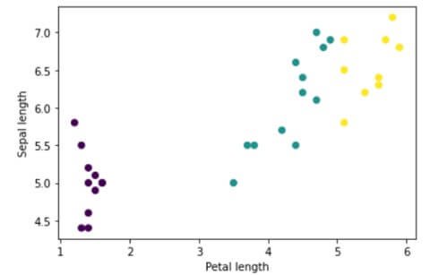
Image 1: Clusters of features
Next, we are going to create a model, named IrisModel, that has three hidden Dense layers.
The activation function determines the output shape of each node in the layer. These non-linearities are important-without them, the model would be equivalent to a single layer. There are many available activations, but ReLU is common for hidden layers.
The ideal number of hidden layers and neurons depends on the problem and the dataset. Like many aspects of machine learning, picking the best shape of the neural network requires a mixture of knowledge and experimentation.
As a rule of thumb, increasing the number of hidden layers and neurons typically creates a more powerful model, which requires more data to train effectively.
Next, we are going to use the model on our data.
The output is:
[[ 2.5031486, -0.22217305, 0.6405254],
[ 2.057041, -0.14333647, 0.5058617],
[ 1.5384593, -0.071346685, 0.36170575],
[ 2.5841222, -0.29190755, 0.691428],
[ 2.4965959, -0.32670006, 0.6901549]]
Here are the predictions, converted to probabilities:
The output is:
[[ 0.8191417, 0.053674366, 0.12718388],
[ 0.75599545, 0.08373507, 0.1602694],
[ 0.6630401, 0.13255922, 0.20440063],
[ 0.82848436, 0.046691786, 0.12482388],
[ 0.81722885, 0.048551414, 0.13421974]]
We can do the predication by class with the following code:
The output is:
Prediction: [0, 0, 0, 0, 0, 0, 0, 0, 0, 0, 0, 0, 0, 0, 0, 0, 0, 0, 0, 0, 0, 0, 0, 0, 0, 0, 0, 0, 0, 0, 0, 0]
Labels: [1, 1, 0, 2, 2, 1, 2, 2, 2, 1, 2, 0, 1, 0, 0, 1, 0, 1, 1, 2, 0, 1, 0, 1, 2, 0, 0, 2, 0, 0, 1, 1]
These results are good because we haven’t trained our model yet.
Both training and evaluation stages need to calculate the model’s loss. This measures how off a model’s predictions are from the desired label, in other words, how bad the model is performing. We want to minimize, or optimize, this value.
Our model will calculate its loss using the softmaxCrossEntropy(logits:labels:) function which takes the model’s class probability predictions and the desired label and returns the average loss across the examples.
Let’s calculate the loss for the current untrained model:
The output is:
Loss test: 1.7008568
To optimize the loss, as the situation suggests, we need to create an optimizer. An optimizer applies the computed gradients to the model’s variables to minimize the loss function.
You can think of the loss function as a curved surface (see Figure 3) and we want to find its lowest point by walking around. The gradients point in the direction of the steepest ascent-so we’ll travel the opposite way and move down the hill.
By iteratively calculating the loss and gradient for each batch, we’ll adjust the model during training. Gradually, the model will find the best combination of weights and bias to minimize loss. And the lower the loss, the better the model’s predictions.
Swift for TensorFlow has many optimization algorithms available for training. This model uses the SGD optimizer that implements the stochastic gradient descent (SGD) algorithm.
The learningRate sets the step size to take for each iteration down the hill. This is a hyperparameter that you’ll commonly adjust to achieve better results.
The output is:
Current loss: 1.7008568
Next, we pass the gradient that we just calculated to the optimizer, which updates the model’s differentiable variables accordingly:
The output is:
Next loss: 1.5416806
With all the pieces in place, the model is ready for training! A training loop feeds the dataset examples into the model to help it make better predictions. The following code block sets up these training steps:
- Iterate over each epoch. An epoch is one pass through the dataset.
- Within an epoch, iterate over each batch in the training epoch
- Collate the batch and grab its features (x) and label (y).
- Using the collated batch’s features, make a prediction, and compare it with the label. Measure the inaccuracy of the prediction and use that to calculate the model’s loss and gradients.
- Use gradient descent to update the model’s variables.
- Keep track of some stats for visualization.
- Repeat for each epoch.
The epochCount variable is the number of times to loop over the dataset collection. Counter-intuitively, training a model longer does not guarantee a better model. epochCount is a hyperparameter that you can tune. Choosing the right number usually requires both experience and experimentation.
This is the output:
Epoch 0: Loss: 1.2862605, Accuracy: 0.40625
Epoch 50: Loss: 0.54648876, Accuracy: 0.7708333
Epoch 100: Loss: 0.3795154, Accuracy: 0.90625
Epoch 150: Loss: 0.27226007, Accuracy: 0.9479167
Epoch 200: Loss: 0.22806416, Accuracy: 0.9895833
Epoch 250: Loss: 0.16147493, Accuracy: 0.9895833
Epoch 300: Loss: 0.14311497, Accuracy: 0.9895833
Epoch 350: Loss: 0.13072757, Accuracy: 0.9791667
Epoch 400: Loss: 0.11862741, Accuracy: 0.96875
Epoch 450: Loss: 0.08667142, Accuracy: 0.9895833
While it’s helpful to print out the model’s training progress, it’s often more helpful to see this progress. We can create basic charts using Python’s matplotlib module.
Interpreting these charts takes some experience, but you really want to see the loss go down and the accuracy goes up.
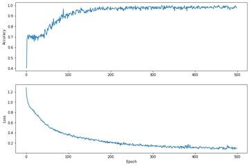
Image 2: Accuracy and Loss per Epoch


After the training part, we have to continue to the testing part. Evaluating the model is similar to training the model. The biggest difference is the examples come from a separate test set rather than the training set.
To fairly assess a model’s effectiveness, the examples used to evaluate a model must be different from the examples used to train the model.
The setup for the test dataset is similar to the setup for the training dataset.
Unlike the training stage, the model only evaluates a single epoch of the test data. In the following code cell, we iterate over each example in the test set and compare the model’s prediction against the actual label.
This is used to measure the model’s accuracy across the entire test set.
The output is:
Test batch accuracy: 0.96666664
We can use the first batch to see if the model is correct.
The outout is:
[1, 2, 0, 1, 1, 1, 0, 2, 1, 2, 2, 0, 2, 1, 1, 0, 1, 0, 0, 2, 0, 1, 2, 2, 1, 1, 0, 1, 2, 1]
[1, 2, 0, 1, 1, 1, 0, 2, 1, 2, 2, 0, 2, 1, 1, 0, 1, 0, 0, 2, 0, 1, 2, 1, 1, 1, 0, 1, 2, 1]
The Final is to see how our trained model works in real life. We’ve trained a model and demonstrated that it’s good-but not perfect-at classifying iris species. Now let’s use the trained model to make some predictions on unlabeled examples; that is, on examples that contain features but not a label.
In real-life, the unlabeled examples could come from lots of different sources including apps, CSV files, and data feeds. For now, we’re going to manually provide three unlabeled examples to predict their labels. Recall, the label numbers are mapped to a named representation as:
- 0: Iris setosa
- 1: Iris versicolor
- 2: Iris virginica
The output is:
Example 0 prediction: Iris setosa ([ 0.9927578, 0.007242134, 1.7388968e-09])Example 1 prediction: Iris versicolor ([0.0024022155, 0.9451288, 0.052468948])Example 2 prediction: Iris virginica ([2.51921e-05, 0.09485072, 0.9051241])
Conclusion
This is just an example of how powerful is Swift paired with TensorFlow. If you are familiar with Swift development, you can pair it up with TensorFlow and make amazing apps for every Apple device.
This sounds very challenging and exciting since there are predictions that the mobile apps market will worth more than $400 billion in 2025, so it is good to start now, while you have time, and be ready to cut a big piece from the pie.
Our article is inspired by TensorFlow.
Like with every post we do, we encourage you to continue learning, trying and creating.
Don’t forget to read our latest and similar articles:
- You Can Now Learn for FREE: 9 Courses by Google about Artificial Intelligence, Machine Learning and Data Science
- Top 40 COMPLETELY FREE Coursera Artificial Intelligence and Computer Science Courses
- Unbelievable: You Can Now Build a Natural Language Processing Question Answering System in LESS Than 20 Lines of Code
- This is the Future of Artificial Intelligence: Deep Learning with JavaScript, Node.js, and TensorFlow