Wikipedia: “In statistics, Bayesian linear regression is an approach to linear regression in which the statistical analysis is undertaken within the context of Bayesian inference.
When the regression model has errors that have a normal distribution, and if a particular form of the prior distribution is assumed, explicit results are available for the posterior probability distributions of the model’s parameters.”
The most common interpretation of Bayes’ formula in finance is the diachronic interpretation. This mainly states that over time we learn new information about certain variables or parameters of interest, like the mean return of a time series.
Equation 1 states the theorem formally. Here, H stands for an event, the hypothesis, and D represents the data an experiment or the real world might present. On the basis of these fundamental definitions, we have:
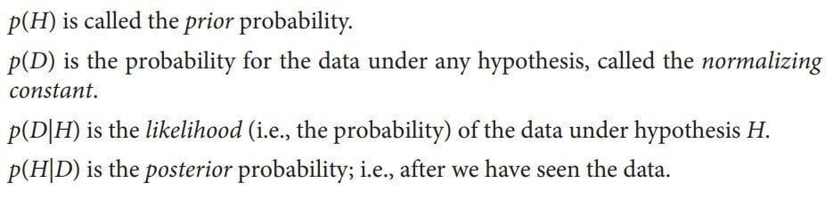
Image 1: Equation 1 parameters
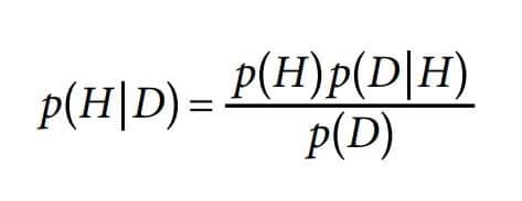
Image 2: Equation 1 – Bayesian Formula
Example: “We have two boxes, B1 and B2. Box B1 contains 20 black balls and 70 red balls, while box B2 contains 40 black balls and 50 red balls. We randomly draw a ball from one of the two boxes.
Assume the ball is black. What are the probabilities for the hypotheses “H1: Ball is from box B1” and “H2: Ball is from box B2,” respectively? Before we randomly draw the ball, both hypotheses are equally likely.
After it is clear that the ball is black, we have to update the probability for both hypotheses according to Bayes’ formula. Consider hypothesis H1”:

Image 3: Solving the example
This gives for the updated probability of H1 p(H1|D) = (0.5·0.2)/0.3 = 1/3. This result also makes sense intuitively. The probability for drawing a black ball from box B2 is twice as high as for the same event happening with box B1.
Therefore, having drawn a black ball, the hypothesis H2 has with p(H2|D) = 2/3 an updated probability two times as high as the updated probability for hypothesis H1.
This example just needs to show you, how you can use Bayesian Regression, and what types of problems you can solve with it on paper.
In this article, we are going to explain to you, how to implement Bayesian Regression using Python, and make your life easier.
Our article is inspired by the book Python for Finance: Mastering Data-Driven Finance that you can buy from Amazon:

Python for Data Analysis: Data Wrangling with Pandas, NumPy, and IPython
This is just another article in our series where we are trying to implement financial problems using Machine Learning and Python. You can also check our other articles:
- Finance with Python: Monte Carlo Simulation (The Backbone of DeepMind’s AlphaGo Algorithm)
- Finance with Python: Convex Optimization
Implement Bayesian Regression using Python
To implement Bayesian Regression, we are going to use the PyMC3 library. If you have not installed it yet, you are going to need to install the Theano framework first. However, it will work without Theano as well, so it is up to you.
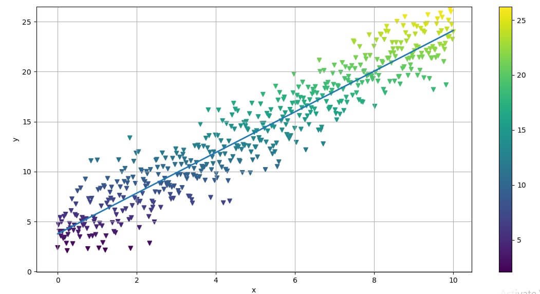
Image 4: Plotting the Linear Regression
This example is a noisy data around a straight line given with the equation
y = 4 + 2 * x + np.random.standard_normal(len(x)) * 2
in the code above.
The regression is implemented using the polyfit() method with the NumPy library.
Note that the highest-order monomial factor (in this case, the slope of the regression line) is at index level 0 and that the intercept is at index level 1. The original parameters 2 and 4 are not perfectly recovered, but this of course is due to the noise included in the data.
Next, the Bayesian regression. Here, we assume that the parameters are distributed in a certain way. For example, consider the equation describing the regression line ŷ(x) = 𝛼 + 𝛽 · x. We now assume the following priors:
- 𝛼 is normally distributed with mean 0 and a standard deviation of 20.
- 𝛽 is normally distributed with mean 0 and a standard deviation of 20.
For the likelihood, we assume a normal distribution with a mean of ŷ(x) and a uniformly distributed standard deviation between 0 and 10. A major element of Bayesian regression is (Markov Chain) Monte Carlo (MCMC) sampling.
In principle, this is the same as drawing balls multiple times from boxes, as in the previous simple example—just in a more systematic, automated way. For technical sampling, there are three different functions to call:
- find_MAP finds the starting point for the sampling algorithm by deriving the local maximum a posteriori point.
- NUTS implements the so-called “efficient No-U-Turn Sampler with dual averaging” (NUTS) algorithm for MCMC sampling given the assumed priors.
- sample draws a number of samples given the starting value from find_MAP and the optimal step size from the NUTS algorithm.
With the code above, we wrap up everything we’ve mentioned within a “with” statement.
Output:
{‘alpha’:3.8783781152509031, ‘beta’: 2.0148472296530033, ‘sigma’: 2.0078134493352975}


Above is the output from the first sample.
All three values are rather close to the original values (4, 2, 2). However, the whole procedure yields, of course, many more estimates.
They are best illustrated with the help of a trace plot, as in Image 5 i.e., a plot showing the resulting posterior distribution for the different parameters as well as all single estimates per sample. The posterior distribution gives us an intuitive sense of the uncertainty in our estimates.

Image 5: Trace plots
Taking only the alpha and beta values from the regression, we can draw all resulting regression lines as shown in the code result and visually in Image 6.
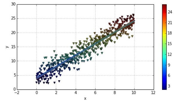
Image 6: Plotting the Bayesian Regression
Conclusion
Bayesian statistics in general (and Bayesian regression in particular) has become a popular tool in finance, as well as in Artificial Intelligence and its subfields since this approach overcomes shortcomings of other approaches.
Even if the mathematics and the formalism are more involved, the fundamental ideas like the updating of probability/distribution beliefs over time are easily grasped intuitively.
We highly recommend you try this on your own, especially if you are learning statics or working in finance, it will help you a lot.
If you are into finance and want to know how to implement Machine Learning and Python in your work we will recommend you our articles about:
- Finance with Python: Monte Carlo Simulation (The Backbone of DeepMind’s AlphaGo Algorithm)
- Finance with Python: Convex Optimization
Like with every post we do, we encourage you to continue learning, trying, and creating.