
A Support Vector Machine (SVM) is a very powerful and versatile Machine Learning model, capable of performing linear or nonlinear classification, regression, and even outlier detection. It is one of the most popular models in Machine Learning, and anyone interested in Machine Learning should have it in their toolbox.
SVMs are particularly well suited for the classification of complex but small or medium-sized datasets.
Wikipedia: “More formally, a support vector machine constructs a hyperplane or set of hyperplanes in a high or infinite-dimensional space, which can be used for classification, regression, or other tasks like outlier detection.
Intuitively, a good separation is achieved by the hyperplane that has the largest distance to the nearest training-data point of any class (so-called functional margin), since in general the larger the margin, the lower the generalization error of the classifier.”
In this article, we are going to show you how to implement Linear Support Vector Machine using Python, as well as help you to understand SVMs.
How to implement Linear Support Vector Machine in Python

Image 1: Linearly separable problem
On Image 1 the two classes can clearly be separated easily with a straight line (they are linearly separable). The left plot shows the decision boundaries of three possible linear classifiers. The model whose decision boundary is represented by the dashed line is so bad that it does not even separate the classes properly.
The other two models work perfectly on this training set, but their decision boundaries come so close to the instances that these models will probably not perform as well on new instances.
In contrast, the solid line in the plot on the right represents the decision boundary of an SVM classifier, this line not only separates the two classes but also stays as far away from the closest training instances as possible.
You can think of an SVM classifier as fitting the widest possible street (represented by the parallel dashed lines) between the classes. This is called a large margin classification.
If we strictly impose that all instances be off the street and on the right side, this is called hard margin classification. There are two main issues with hard margin classification. First, it only works if the data is linearly separable, and second, it is quite sensitive to outliers.
Image 2 shows the iris dataset with just one additional outlier: on the left, it is impossible to find a hard margin, and on the right, the decision boundary ends up very different from the one we saw in Image 1 without the outlier, and it will probably not generalize as well.
To avoid these issues, it is preferable to use a more flexible model. The objective is to find a good balance between keeping the street as large as possible and limiting the margin violations (i.e., instances that end up in the middle of the street or even on the wrong side). This is called a soft margin classification.
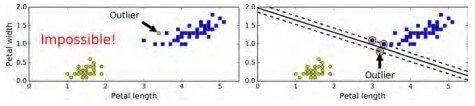
Image 2: Hard Margin Classification issue
In Scikit-Learn’s SVM classes, you can control this balance using the C hyperparameter: a smaller C value leads to a wider street but more margin violations.
Image 3 shows the decision boundaries and margins of two soft margin SVM classifiers on a nonlinearly separable dataset. On the left, using a high C value the classifier makes fewer margin violations but ends up with a smaller margin. On the right, using a low C value the margin is much larger, but many instances end up on the street.
However, it seems likely that the second classifier will generalize better: in fact, even on this training set, it makes fewer prediction errors since most of the margin violations are actually on the correct side of the decision boundary.
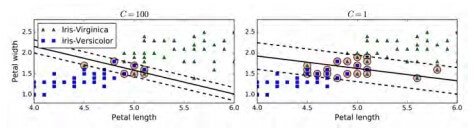
Image 3: Margin violations based on the C hyperparameter
Below is a Python code of how to implement Linear SVMs.
The prediction results in class 0 or 1 for the pairs.
The output is:
The classes are: [1. 1. 0.]
If we set C=10 we get the next output:
The classes are: [1. 0. 0.]
Larger C value, smaller margin, and we have a different classification, now, the last two belong to the same class.
Conclusion
SVMs are very powerful tools if you are using them the right way. We’ve seen examples on other websites and platforms where people explain linear and nonlinear SVMs in one article but we think that in order to help you understand it better we will focus on one at the time. In the future, we will make an article on nonlinear SVMs.
If you are new to Machine Learning, Deep Learning, Computer Vision, Data Science or just Artificial Intelligence, in general, we will suggest you some of our other articles that you might find helpful, like:
- FREE Computer Science Curriculum From The Best Universities and Companies In The World
- How To Become a Certified Data Scientist at Harvard University for FREE
- How to Gain a Computer Science Education from MIT University for FREE
- Top 10 Best FREE Artificial Intelligence Courses from Harvard, MIT, and Stanford
- Top 10 Best Artificial Intelligence YouTube Channels in 2020
Like with every post we do, we encourage you to continue learning, trying and creating.