Monte Carlo simulation is one of the most important algorithms in finance and numerical science in general. Its importance stems from the fact that it is quite powerful when it comes to option pricing or risk management problems.
In comparison to other numerical methods, the Monte Carlo method can easily cope with high-dimensional problems where the complexity and computational demand, respectively, generally increase in a linear fashion. (Read Effortless Way To Implement Linear Regression in Python)
The downside of the Monte Carlo method is that it is computationally demanding and often needs huge amounts of memory even for quite simple problems.
In this article, we are going to implement a Monte Carlo simulation using pure Python code. We decided to use Python since it is very popular among the Machine Learning community and it increases its popularity in the Finance community.
Here’s a new Finance with Python article where you will learn about Convex Optimization.
Implementing a Monte Carlo Simulation using Python Programming Language
The example that follows illustrates different implementation strategies in Python and offers three different implementation approaches for a Monte Carlo-based valuation of a European option.
The examples are based on the model economy of Black-Scholes-Merton, where the risky underlying stock price or index level) follows, under risk neutrality, a geometric Brownian motion with a stochastic differential equation (SDE)
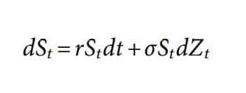
Formula 1: Black-Scholes-Merton stochastic differential equation
Formula 1 comes by combining Formula 2 (below) and the Brownian motion (Z)

Formula 2: Black-Scholes-Merton option pricing formula
The parameters of Formula 2 are explained below.

Image 1: Black-Scholes-Merton option pricing formula parameters
There is also a discretization of the SDE done by Euler with the formula below.
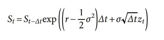
Formula 3: Euler discretization of the SDE
The variable z is a standard normally distributed random variable, 0 < Δt < T, a time interval. It also holds 0 < t ≤ T with T the final time horizon.
With the code above we are calculating the exact value of the option.
This is our benchmark value for the Monte Carlo estimators to follow. To implement a Monte Carlo valuation of the European call option, the following recipe can be applied:
- Divide the time interval [0,T] in equidistant subintervals of length Δt.
- Start iterating i = 1, 2,…, I.
a) For every time step t ∈ {Δt, 2Δt,…, T}, draw pseudorandom numbers zt (i).
b) Determine the time T value of the index level ST(i) by applying for the pseudorandom numbers time step by time step to the discretization scheme in Formula 3.
c) Determine the inner value hT of the European call option at T as hT(ST(i)) = max(ST(i) – K,0).
d) Iterate until i = I.
3. Sum up the inner values, average, and discount them back with the riskless short rate according to Formula 4. Formula 4 provides the numerical Monte Carlo estimator for the value of the European call option.

Formula 4: Monte Carlo Estimator for European Call Function
European Option Value: 7.999044888176586
Duration in Seconds: 36.534881591796875
As you can see the program took almost 37 seconds and predicted value equal to around 8 which is really close to our benchmark.
Note that the estimated option value itself depends on the pseudorandom numbers generated while the time needed is influenced by the hardware the script is executed on.
European Option Value: 8.00445606947662
Duration in Seconds: 39.818453311920166
This is the output if we generate 50000 numbers. (seed(20000))
There are more efficient and ways to predict the value of the option that we are going to discuss in some of the upcoming posts.
Conclusion
Python is one of the most popular languages in the world since it has easy to understand syntax and has tons of powerful libraries for application development and Artificial Intelligence (Machine Learning, Deep Learning, Computer Vision, NLP, Reinforcement Learning, etc).
Getting this popularity, it makes the language to be the number one choice in many other fields where Information Technology is making its way, like finance, medicine, etc.
We hope you will find this helpful especially if you are working in finance and you have not programming experience.
Don’t forget to read the previous blog post: Most Important Keyboard Shortcuts for Windows That Will Save You Time
Like with every post we do, we encourage you to continue learning, trying and creating.