If you’ve ever read anything related to data science, machine learning or data mining, there is a high probability of you coming across clustering.
Clustering is a process of classifying data in clusters based on how similar the data is. There are many clustering algorithms. One of the most known is the K-means algorithm.
K-means clusters the data into a determined number of clusters. Each observation of the data belongs to the cluster with the nearest mean, serving as a prototype to the cluster.
K-means minimizes within-cluster variances (squared Euclidean distances), but not regular Euclidean distances, which would be the more difficult Weber problem: the mean optimizes squared errors, whereas only the geometric median minimizes Euclidean distances.
Image color quantization using K-means
In the next example, we are going to show you how can you use K-means clustering in image color quantization. To implement K-means in image color quantization we are going to use the OpenCV library.
Color quantization is the process of reducing the number of colors in an image. One reason to do so is to reduce memory. Sometimes, some devices have limitations such that it can produce only a limited number of colors. In cases like this, we can use color quantization.
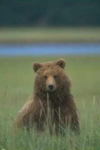
Image 1: The image used in the example
import numpy as np
import cv2
Importing the two libraries we need in this example. The first one is numpy which is used so we can do manipulations with multidimensional structures. The second is OpenCV.
img = cv2.imread(‘example2.jpg‘)
Z = img.reshape((-1,3))
Z = np.float32(Z)
Then we are reading the image, and we are reshaping it in Mx3 shape (M is the number of rows, 3 is a number of rows, also representing the three channels Red, Blue and Green (RGB) which are the features we are going to use in order to do color quantization). Then we are converting the image pixel values into float32 type, because it is the only format that the kmeans method can use as a source.
criteria = (cv2.TERM_CRITERIA_EPS + cv2.TERM_CRITERIA_MAX_ITER, 10, 1.0)
K = 3
ret,label,center=cv2.kmeans (Z,K,None,criteria,10,cv2.KMEANS_RANDOM_CENTERS)
The k-means method takes a few input parameters. As we can see from the last line in the code above, it takes an image, where the pixels are in float32 format, then intakes the number of kernels we want to have for the image. We decided to have three because we are using three features for the quantization.
The argument with value None is for the output image, but we are not using it here. Then we have the criteria, which is defined in the first line of the code above. We can see, that it is a tuple of three values. The first is a type of termination, which here contain two criteria.
The first one stops the algorithms if the defined precision epsilon is reached, and the second stop the algorithm if the specified number of iterations is met. In this case, the algorithm will stop when at least one of the criteria is being met.
The second value is the maximum number of iterations, and the third is the epsilon parameter which is the precision. The fifth argument is the number of attempts that the algorithm is going to be executed. The last argument is used to specify how initial centers are taken.
In the last line of the code above, we can see that we get three outputs, the first one is the compactness (the sum of squared distance from each point to their corresponding center), the second is the labels (every pixel is marked with the corresponding label) and the third is the centers (array of clusters centers).
center = np.uint8(center)
res = center[label.flatten()]
res2 = res.reshape((img.shape))
With the code above, we are casting the float32 values for the centers, into uint8, and shaping the result into the same shape of the source image in order to display it.
cv2.imshow(‘res2‘,res2)
cv2.waitKey(0)
cv2.destroyAllWindows()
With this code, we are displaying the result.
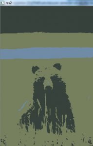
Image 2: Result of the clustering
On Image 2 is represented the result of the clustering. As we can see, there are 3 colors of pixels that image gets, and those represent the three clusters that we’ve chosen to have.
The number of colors, or clusters can change if we change the value that the “K” parameter has. The results of changing the value are shown in the picture below.
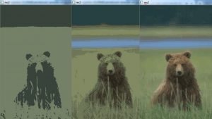
Image 3: Comparison of the results after changing the number of clusters
Conclusion
This post is just an example of how can you use clustering techniques in image processing. There are many other algorithms that you can use, so you can get better results.
We hope that we spark a little interest in you so you will be learning more about image processing and how can you combine it with other techniques.
Like with every post we do, we encourage you to continue learning, trying and creating.