How To Predict Happiness Index Using Machine Learning Model

The World Happiness Report is an annual publication of the United Nations Sustainable Development Solutions Network. It contains articles and rankings of national happiness based on respondent ratings of their own lives, which the report also correlates with various life factors.

In this article, we are going to create a Machine Learning model that will predict happiness index based on the GDP that the world countries have.

Our article is inspired by the book:

Hands-On Machine Learning with Scikit-Learn, Keras, and TensorFlow: Concepts, Tools, and Techniques to Build Intelligent Systems by Aurélien Géron.

We modified the example and the output so we could have our print, and our version of the solution.

The data is from 2015.

Predicting the happiness index

For this problem, there are two datasets in the book, but we are going to use three. So the datasets we are going to use are: IMF(GDP by countries), OECD(happiness index of OECD members), and WHR2015 (happiness index of every country).

You can also find the first two datasets following this link. We are going to combine the first two datasets and we are going to use them in the training of our model, and then we are going to make predictions.

The predictions that we made, we are going to compare to the actual index that you will find in WHR2015 dataset, since that is very precisely calculated taking in count many other variables.

import matplotlib.pyplot as plt
import numpy as np
import pandas as pd
from sklearn.linear_model import LinearRegression

With the code above, you can see the libraries used in for this problem. The matplotlib is used for plotting(visualizing) the results, numpy for high dimensional arrays manipulation, pandas for creating data-frames from the input sources and scikit-learn for using statistics in order to create the Machine Learning model.

Next, we read the data and we organize it in order to be understandable for us, and for our model.

oecd_bli = pd.read_csv(“oecd_bli_2015.csv”, thousands=‘,’)
gdp_per_capita = pd.read_csv(“gdp_per_capita.csv”,thousands=‘,’,delimiter=‘\t‘,
encoding=‘latin1’, na_values=“n/a”)
gdp_per_capita_copy = gdp_per_capita.copy()

We create copies from the data because we are going to need pure data later on.

country_stats = prepare_country_stats(oecd_bli, gdp_per_capita)

X = np.c_[country_stats[“GDP per capita”]]
y = np.c_[country_stats[“Life satisfaction”]]

Next, we create a data-frame combining the two previous data-frames using a custom function (you can see the code below). And we are going to create our features (the GDP per capita in variable X) and our labels (Life satisfaction in variable Y)

def prepare_country_stats(oecd_bli, gdp_per_capita):
oecd_bli = oecd_bli[oecd_bli[“INEQUALITY”] == “TOT”]

oecd_bli = oecd_bli.pivot(
index=“Country”, columns=“Indicator”, values=“Value”)

gdp_per_capita.rename(columns={“2015”: “GDP per capita”}, inplace=True)
gdp_per_capita.set_index(“Country”, inplace=True)
full_country_stats = pd.merge(left=oecd_bli, right=gdp_per_capita,
left_index=True, right_index=True)
full_country_stats.sort_values(by=“GDP per capita”, inplace=True)
remove_indices = [0, 1, 6, 8, 33, 34, 35]
keep_indices = list(set(range(36)) – set(remove_indices))

return full_country_stats[[ “GDP per capita”, ‘Life satisfaction’]].iloc[keep_indices]

With the code above we implement the custom function prepare_country_stats(). As arguments, it uses the two datasets in the form of a data frame.

We set the inequality to “TOT” (which means TOTAL, taking in count the low, high, female and male inequality for the OECD countries), we set the “Country” column to be our index.

We do the same for the GDP’s dataset except for instead of counting we change the name of the “2015” column to “GDP per capita” since it is more understandable.

The result is a data-frame that has an index (which is country) and two columns, one for the GDP, the other for the Life satisfaction).

model = LinearRegression()
model.fit(X, y)

Then we create the model, in this case, the Linear Regression model. If you want to see how to implement Linear Regression in Python yourself following its mathematical equations you can check out our article about Effortless Way To Implement Linear Regression in Python.

After that, we train the model.

checked_countries=[]
prediction_features=[]
prediction_countries = [“Togo” ,“FYR Macedonia”, “Switzerland”, “India”, “Mexico”, “Norway”]

for index,row in gdp_per_capita_copy.iterrows():
for pc in prediction_countries:
if pc not in checked_countries:
if row[‘Country’] == pc:
prediction_features.append([row[“Country”], row[“2015”]])
checked_countries.append(pc)

With the code above, we took the GDP values for countries that are unknown for the model, i.e. countries that were not in the training set. We are going to predict the happiness index for these countries.

actual_values = [[“India”, 4.565], [“FYR Macedonia”, 5.007], [‘Mexico’, 7.187], [‘Norway’, 7.522], [‘Switzerland’, 7.587], [“Togo”,2.839]]

We also create a list of the actual values, that we take from the WHR2015 dataset.

prediction_results=[]
for pf in prediction_features:
predict = model.predict([[pf[1]]])
prediction_results.append([pf[0], round(predict[0][0],3)])

After this, with the code above we make the predictions, and we organize the data in a new list.

labels = [prediction_results[0][0], prediction_results[1][0], prediction_results[2][0], prediction_results[3][0], prediction_results[4][0], prediction_results[5][0]]
predict_plot = [prediction_results[0][1], prediction_results[1][1], prediction_results[2][1], prediction_results[3][1], prediction_results[4][1],prediction_results[5][1]]
actual_plot = [actual_values[0][1],actual_values[1][1],actual_values[2][1],actual_values[3][1],actual_values[4][1],actual_values[5][1]]
x = np.arange(len(labels))
width = 0.35

fig, ax = plt.subplots()
rects1 = ax.bar(x – width/2, predict_plot, width, label=‘Predicted indexes’)
rects2 = ax.bar(x + width/2, actual_plot, width, label=‘Actual indexes’)

autolabel(rects1)
autolabel(rects2)
ax.set_ylabel(‘Indexes’)
ax.set_title(‘Prediction versus Actual happiness index’)
ax.set_xticks(x)
ax.set_xticklabels(labels)
ax.legend()
fig.tight_layout()
plt.show()

def autolabel(rects):

for rect in rects:
height = rect.get_height()
ax.annotate(‘{}’.format(height),
xy=(rect.get_x() + rect.get_width() / 2, height),
xytext=(0, 3),
textcoords=“offset points”,
ha=‘center’, va=‘bottom’)

Next, we plot the data using the matplotlib library, and custom autolabel() function. Here you can find a detailed explanation for the plotting.

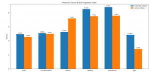
Results of the happiness index prediction versus the actual values

Image 1: Results of the prediction versus the actual values

On Image 1, you can see the results of the prediction index values versus the actual index values. We have 6 countries in total.

We have poor countries like Togo, middle counties like India and North Macedonia, and top 20 counties like Mexico, Switzerland and Norway.

We can see that predicted index is quite different in from the actual index in the poor countries like Togo, since it is also a dictatorship, where freedom of speech, women’s and minorities rights are suppressed, and since there are not a lot of money, the major human rights are more essential.

We can see that this is a case in highly developed countries like Mexico, Switzerland and Norway. Their people enjoy more things and they can afford enough with their salaries, so obviously some other things are going to have an impact on people’s happiness.

In the middle countries, we can see that the happiness index, is highly influenced by the GDP, which translates that the economic conditions in those countries have a huge impact on the happiness index.

Culturally different, India and North Macedonia have one thing in common and that is the rise of foreign investments, and that means a huge flow of money, opening new work positions for the population, and shifting the economic situation of their people, which translate to valuating different things.

Conclusion

This article should not be used as a conclusion for any country, because each of the countries has a huge cultural heritage, and that is what we should value first.

This article is just an example of how broad is the usage of Machine Learning, and what we can achieve if we are using it in the right way.